Hyperplane Intuition
In studying SVMs, I encountered hyperplanes. In this post we’ll work on developing a basic intuition about hyperplanes. At the bottom of this post I pasted all of the Python I used in these explorations as well as a summary of the intuition gained.
Hyperplanes, Subspaces, And Ambient Spaces
According to wikipedia, a hyperplane is “a subspace whose dimension is one less than that of its ambient space.”
A subspace is wholly contained in another space, or whose points or elements are all in another space. An ambient space is the space surrounding a “mathematical object,” where these objects are anything that can be defined mathematically.
We can think of a given line – a 1-dimensional mathematical object – as both
- an ambient space of any single point on that line
- a subspace of (one of) the plane(s) of which it is part.
Similarly, we can think of a given plane – a 2-dimensional mathematical object – as both
- an ambient space of any of an infinity of lines parallel to the plane
- a subspace of a 3-dimensional space.
Equation For A Hyperplane
Given the equation for a hyperplane
\begin{equation} H_0 = \vec{w} \cdot \vec{x} + b = 0, \end{equation}
where \(H_0\) is the hyperplane that specifies our SVM’s decision boundary, let’s develop an intuition for varying the weight vector \(w\) and the bias \(b\) (which could be written as part of \(w\) if we considered every training example vector \(x\) to have an additional \(x_0 = 1\)).
Given this 2-d hyperplane, if we consider the 3-dimensional space of which it is a subspace, we can imagine different values of \(x_1, x_2\) such that for all \(x\) where \(\vec{w} \cdot \vec{x} > 0\) the model will classify one class (say, the positive class), and otherwise the model will predict the other class (say, the negative class). The cutoff is at 0 because \(H_0 = 0\).
What Is A Hyperplane?
A hyperplane is a particular subspace whose dimension is 1 less than the space its in. The hyperplane divides its ambient space into two pieces – as when a point divides a line or a plane divides 3-dimensional space. We’ll look at the latter example in more detail below.
As in other ML algorithms, we’ll presumably be varying the weight vector \(\vec{w}\) in the process of optimizing something – in SVMs we’re searching for the optimal hyperplane \(H_0\) to separate our data (we’ll look at this algorithm and what “optimal” means in the next post).
The Setup
In order to work with a 2-dimensional hyperplane in 3-space, let’s assume we have a training set of \(m\) examples having 2 features – such that the third dimension represents the value our SVM will base its prediction on for that training example; if a prediction for a given example \(x_i\) is, in the 3rd dimension, greater than 0, we’ll classify as one class and as the other if not.
We’re interested to gain intuition of the effects on the hyperplane \(H_0\) of varying
- the direction of weight vector \(w\)
- the magnitude of \(w\)
- the value of the bias \(b\)
Direction Of Weight Vector
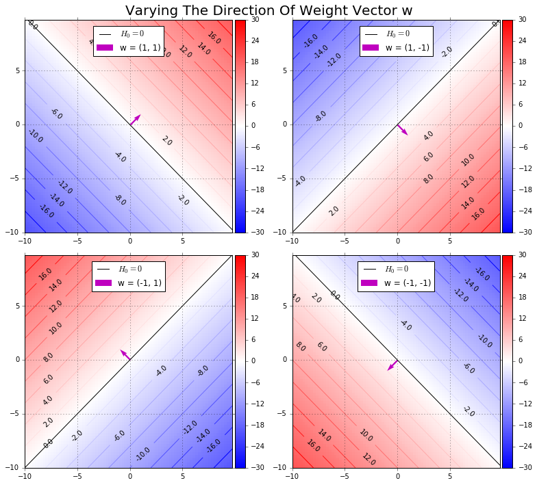
If we orient \(w\) in 4 opposite directions we can note that
- \(w\) is always perpendicular to \(H_0\)
- \(w\) always points in the direction of the class that will be classified as positive (e.g. \(\vec{w} \cdot \vec{x} + b > 0\)).

Magnitude Of Weight Vector
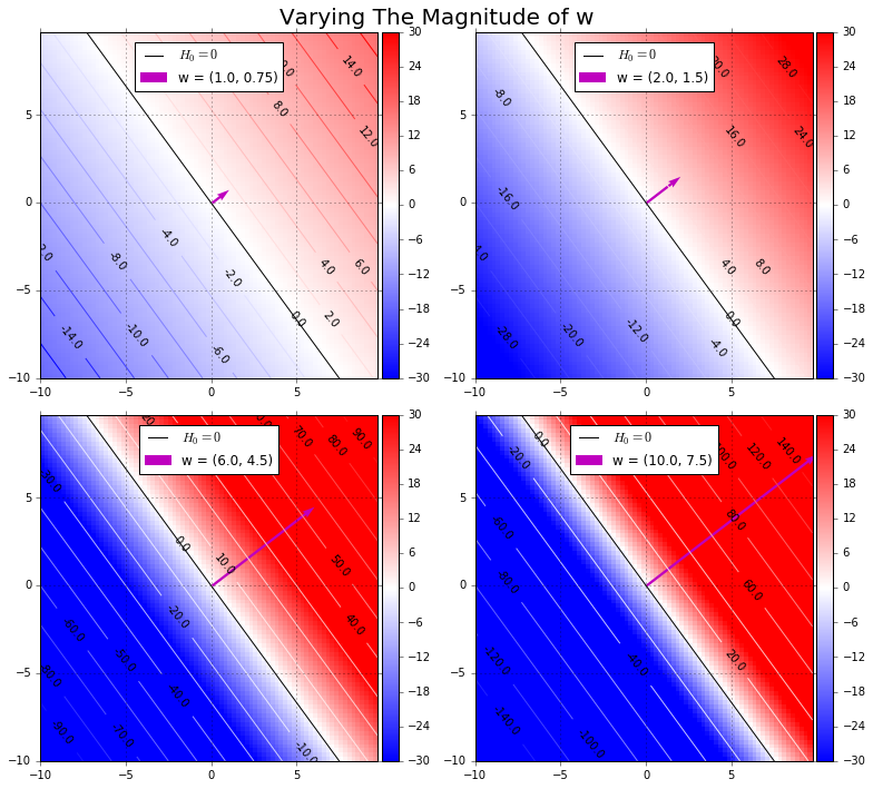
Changing the magnitude of \(w\) we note that
- the position of \(H_0\) does not change. The decision boundary stays in one place. However,
- \(\vec{w} \cdot \vec{x} + b = 1\) and \(\vec{w} \cdot \vec{x} + b = -1\) do shift:
- the higher the magnitude of \(w\) the closer together are these hyperplanes parallel to \(H_0\). These two hyperplanes are important in SVMs (discussed in future post).

Value Of The Bias
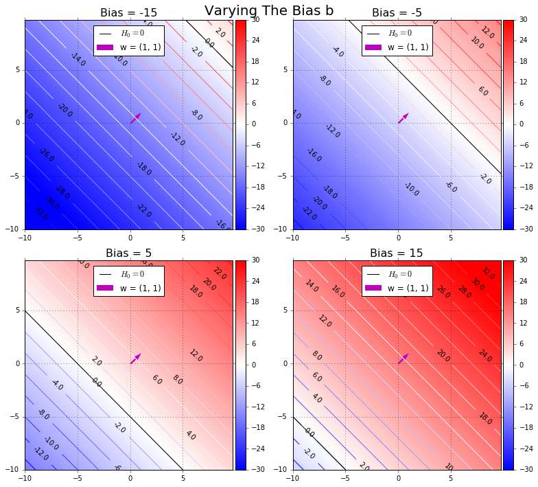
Changing the value of the bias we observe that
- the bias offsets \(H_0\) in a direction parallel to the weight vector \(w\).
- A negative bias requires \(b\) more from \(\vec{w} \cdot \vec{x_i}\) for \(x_i\) to be classified as positive.
- A positive bias requires \(b\) less from \(\vec{w} \cdot \vec{x_i}\) for \(x_i\) to be classified as negative.
- In other words, the bias shifts the boundary in the direction opposite to the sign of the bias.

Summary Of Effects
We can:
- Rotate \(H_0\) by rotating the direction of \(\vec{w}\)
- Move \(H_0\) back and forth along \(\vec{w}\) by setting a positive or negative bias, respectively
- “Squish” \(H_1\) and \(H_2\) (hyperplanes parallel to and on either side of \(H_0\)) closer to \(H_0\) by increasing the magnitude of \(\vec{w}\)
- Conversely, and critically, we maximize the width of the margin (\(m\)) between \(H_1\) and \(H_2\) by minimizing the magnitude of \(\vec{w}\).
Python Code
import numpy as np
import matplotlib.pyplot as plt
from mpl_toolkits.axes_grid1 import make_axes_locatable
%matplotlib inline

def get_XYZ(xlim, ylim, w, b):
    delta = 0.25
    x = np.arange(xlim[0], xlim[1], delta)
    y = np.arange(ylim[0], ylim[1], delta)
    X, Y = np.meshgrid(x, y)
    Z = np.dstack([X,Y]).dot(w) + b
    return (X, Y, Z)

def plot_contour(fig, ax, w=np.array([1, 2]), b=0):
    '''
        Plot a contour plot of X.dot(W) + b = Z
            where w=weight vector w and b=bias
    '''
    # Determine values to plot
    # TODO: variable limits aren't working quite as well as they could,
    # so are currently hard-coded
    xlim=np.array([-10,10])
    ylim=np.array([-10,10])

    X, Y, Z = get_XYZ(xlim, ylim, w, b)

    # Contour Plot
    contour_plot = ax.contour(X, Y, Z, 20, cmap=plt.cm.bwr)

    import matplotlib.colors as colors
    pcm = ax.pcolormesh(X, Y, Z, vmin=-30, vmax=30, cmap='bwr')
    ax.clabel(contour_plot, inline=1, fontsize=10, fmt='%1.1f', colors='k')

    # Set dimensions
    ax.set_xlim(min(x), max(x))
    ax.set_ylim(min(y), max(y))
    ax.grid()

    # Show color bar adjacent to a plot
    divider = make_axes_locatable(ax)
    cax = divider.append_axes("right", size="5%", pad=0.05)
    fig.colorbar(pcm, cax=cax)

    plot_weight_vector(ax, w)
    plot_hyperplane(ax, x, w, b)
    ax.legend(loc='center', bbox_to_anchor=(0.5, 0.90))

def plot_hyperplane(ax, x, w, b):
    ax.plot(x, (-b - w[0]*x)/w[1], color='black', label=r'$H_0 = 0$')

def plot_weight_vector(ax, w):
#   tail = np.array([np.average(xlim), np.average(ylim)])
    tail = np.array([0,0])
    head = tail + w
    soa = np.array([
        [tail[0], tail[1], head[0], head[1]]
    ])
    X, Y, U, V = zip(*soa)
    q = ax.quiver(X, Y, U, V, angles='xy', scale_units='xy', scale=1, color='m', label=f"w = {w[0], w[1]}")
# Varying Weight Direction
weights = np.array([
[(1,1),(1,-1)],
[(-1,1),(-1,-1)]
])
fig, axes = plt.subplots(weights.shape[0], weights.shape[1], figsize=(11, 10))
fig.suptitle("Varying The Direction Of Weight Vector w", fontsize=20)
for index, ax in np.ndenumerate(axes):
plot_contour(fig, ax, weights[index])
plt.tight_layout()
fig.subplots_adjust(top=0.95)
# Varying Weight Magnitude
magnitudes = np.array([
[0.5, 1],
[3, 5]
])
w = np.array([2,1.5])
fig, axes = plt.subplots(bias.shape[0], bias.shape[1], figsize=(11, 10))
fig.suptitle("Varying The Magnitude of w", fontsize=20)
for index, ax in np.ndenumerate(axes):
b = bias[index]
plot_contour(fig, ax, w * magnitudes[index])
plt.tight_layout()
fig.subplots_adjust(top=0.95)
# Varying The Bias
bias = np.array([
[-15, -5],
[5, 15]
])
w = np.array([1,1])
fig, axes = plt.subplots(bias.shape[0], bias.shape[1], figsize=(11, 10))
fig.suptitle("Varying The Bias b", fontsize=20)
for index, ax in np.ndenumerate(axes):
b = bias[index]
plot_contour(fig, ax, w, b)
ax.set_title(f'Bias = {b}', size=16)
plt.tight_layout()
fig.subplots_adjust(top=0.95)