The general form of a confidence interval for any unknown parameter: \begin{equation} \text{estimate} \pm \text{margin of error} \end{equation}

For categorical variables we use the sample proportion \(\hat p\) as the estimator for the population proportion \(p\)

\begin{equation} \hat p \pm m \end{equation}

The margin of error \(m\) breaks down into \begin{equation} m = \text{confidence multiplier} \cdot \text{SD of the estimator} \end{equation}

Given the Central Limit Theorem we know that the sample distribution of \(\hat p\) has a mean of \(p\) (the population proportion) and a standard deviation of

\begin{equation} \sqrt{\frac{p(1 - p)}{n}} \end{equation}

We can’t use \(p\) in our confidence interval formula – that’s the population parameter we’re trying to infer about – so in the formula for standard deviation of \(\hat p\) we replace \(p\) with \(\hat p\), thus working with the standard error \(\sqrt{\frac{\hat p(1 - \hat p)}{n}}\), altogether we have

\begin{equation} \hat p \pm z^* \cdot \sqrt{\frac{\hat p(1 - \hat p)}{n}} \tag{Proportion confidence interval} \end{equation}

As with estimating the mean of a quantitative variable, there is a tradeoff between confidence (high \(z^*\)) and precision of the estimate (interval width).

To achieve greater precision we can also increase the sample size \(n\).

Determining Sample Size

We can determine a sample size that will satisfy a given level of confidence for the interval we will provide. First we select the level of confidence we wish to achieve, i.e. set a value for \(z^*\). For example, for 95% confidence (a commonly used confidence value) \(z^* \approx 2\). This gives us the equation for the margin of error

\begin{equation} m = 2\sqrt{\frac {\hat p(1 - \hat p)} {n} } \end{equation}

which we can isolate for the sample size \(n\)

\begin{equation} n = \frac{4\hat p(1 - \hat p)}{m^2} \end{equation}

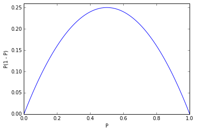
Taking a look at a graph of \(\hat p(1 - \hat p)\)

we see that \(max(\hat p(1 - \hat p))\) for \(0 \le \hat p \le 1\) occurs at \(\hat p = 0.5\); setting this value will maximize the numerator of the equation, thereby giving us the most conservative (largest) estimate for the sample size

Thus we have

\begin{equation} n = \frac{1}{m^2} \tag{Sample size estimate} \end{equation}

as the conservative estimate of the sample size for a 95% confidence interval.

Determining Margin of Error

We can also make the same conservative estimate (using \(\hat p = 0.5\)) for the margin of error (for a 95% confidence interval) given a sample size

\begin{equation} m = \frac{1}{\sqrt{n}} \tag{Margin of error estimate} \end{equation}

such that this estimate will yield the maximum margin of error for any question asked of a random sample with size \(n\), regardless of the particular sample proportions.

Requirements for Methods Used Above

As when the inferring about the mean, the assumption we are making when estimating the proportion is that the sampling distribution of \(\hat p\) is normal. The conditions for when this happens are \(np \ge 10\) and \(n(1 - p) \ge 10\); \(p\) is unknown, so we use the \(\ge 10\) requirement with \(\hat p\) instead.