Bayes' Rule And Conditional Probability
Conditional Probability
- The conditional probability of event \(A\) given event \(B\) can be expressed as \begin{equation} P(A|B) = \frac{P(A \cap B)}{P(B)} \tag{1}\label{1} \end{equation}
- In \eqref{1}, we say that \(A\) is being conditioned by \(B\).
- Note that the Complement Rule extends to conditional probabilities only when you condition on the same event, like this: \begin{equation} P(A|B) + P(A| \neg B) = 1 \end{equation}
Independence Checks
Events \(A\) and \(B\) are independent iff any one of these 4 checks are true. All 4 equations should be true (or all false) for the same reason that we only need three particular values in a probability table to fill out the rest of the values.
\begin{equation} P(B | A) = P(B) \end{equation}
\begin{equation} P(A | B) = P(A) \end{equation}
\begin{equation} P(B | A) = P(B | \neg A) \end{equation}
\begin{equation} P(A \cap B) = P(A) \cdot P(B) \end{equation}
General Multiplication Rule
This rule can be used to find the probability of two events \(A\) and \(B\) both occurring regardless of whether the events are independent.
\begin{equation} P(A \cap B) = P(A) \cdot P(B | A) \tag{2}\label{2} \end{equation}
Notes:
- This rule is a reformulation of \eqref{1}.
- If \(A\) and \(B\) are independent, \(P(B | A) = P(B)\).
- Another formulation of this rule would be
\begin{equation} P(A \cap B) = P(B) \cdot P(A | B) \tag{3}\label{3} \end{equation}
Probability Trees
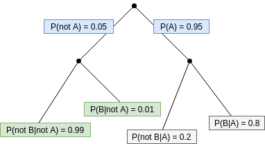
Probability trees can be used to express conditional probabilities.
- Probabilities in the 1st branch-off are non-conditional.
- Any subsequent branch-offs reflect conditional probabilities.
- Probabilities of branches from one point always add up to 1.

Law of Total Probability
In a probability tree, we can find the total probability of some event \(B\) by adding up all of its occurrences via conditional probabilities \begin{equation} P(B) = P(A) \cdot P(B | A) + P(\neg A) \cdot P(B | \neg A). \tag{4}\label{4} \end{equation}
There are sometimes situations where
- we know the ultimate outcome, and
- want to find the probability that a certain event occurred previously.
Bayes’ Rule
If we combine \eqref{1} and \eqref{2} we arrive at Bayes’ Rule
\begin{equation} P(A|B) = \frac{P(B|A) \cdot P(A)}{P(B)}, \tag{5}\label{5} \end{equation} which can be understood as
\begin{equation} Posterior = \frac{Likelihood \cdot Prior}{Evidence} \end{equation}
In the context of prediction
- posterior means the confidence of our prediction \(A\) given evidence \(B\).
- likelihood as in “the likelihood of seeing evidence (i.e. features) \(B\) given a particular class \(A_i\)
- prior refers to the probability of seeing a given class \(A_i\) in our past experience (i.e. in the dataset)
- evidence refers to the probability of seeing a given set of features
- In practice, for the Naive Bayes Classifier (I haven’t gotten to fully implementing this yet, particularly due to the just throw a logarithm around everything solution to the underflow problem), since we are interested in finding the class with the highest probability for a given set of evidence, this term is constant for the calculations for each class and thus cancels out)
A nice introduction to Bayes’ Rule. Bayesian reasoning is about how to revise our beliefs in the light of evidence.
We can also the law of total probability \eqref{4} to \eqref{5} to produce another version of Bayes’ Rule:
\begin{equation}
P(A|B) = \frac{P(B|A) \cdot P(A)}{
P(B | A) \cdot P(A) + P(B | \neg A) \cdot P(\neg A)
} \tag{6}\label{6}
\end{equation}
We can use the above form to solve problems given a probability tree (above).